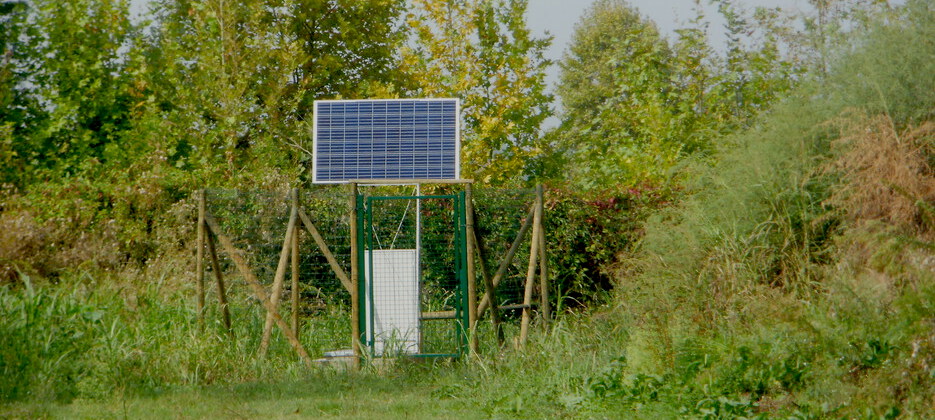
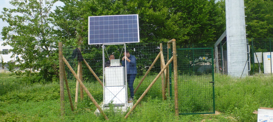
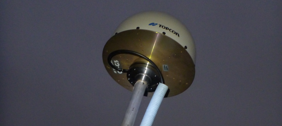
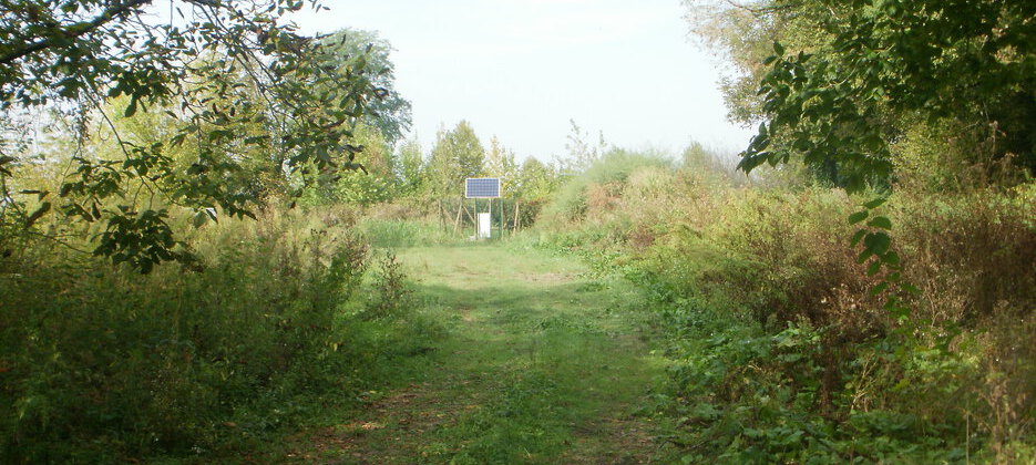
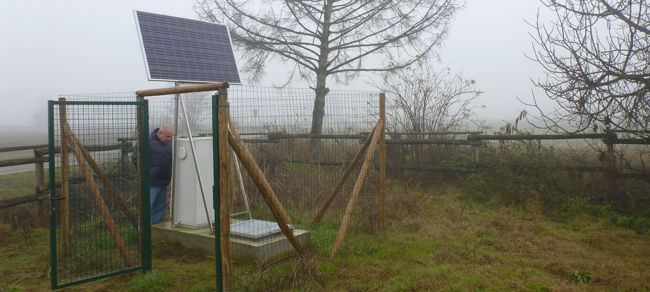
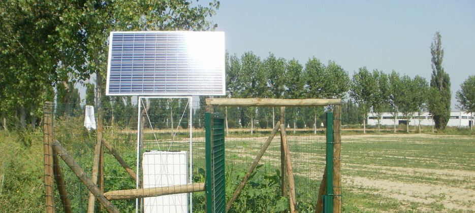
The Cornegliano Laudense Seismic Network (RSCL) consists of nine seismic stations and a permanent precision GNSS-GPS geodetic station focused on the Cornegliano Laudense gas storage reservoir. Seismic monitoring has been active since 1/1/2017.

The RSCL integrates some stations belonging to the regional seismic networks managed by OGS and the Centralized National Seismic Network (RSNC) managed by the National Institute of Geophysics and Volcanology (INGV); in this way, it is possible to detect seismic events, not perceivable by the population, which occur in all directions to a distance of a few tens of kilometres from the storage site.

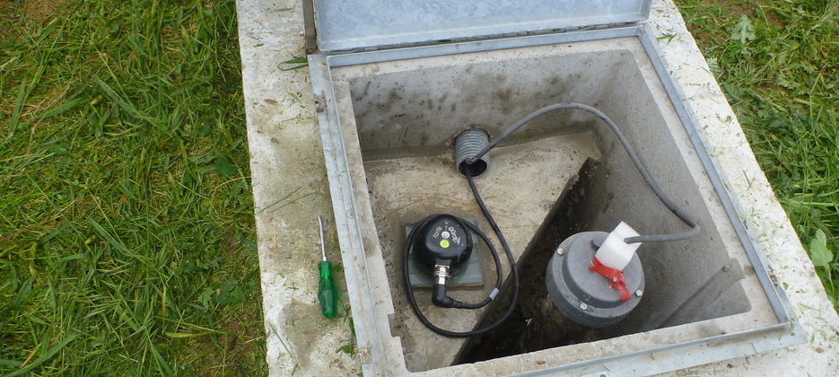
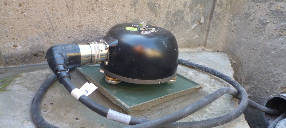
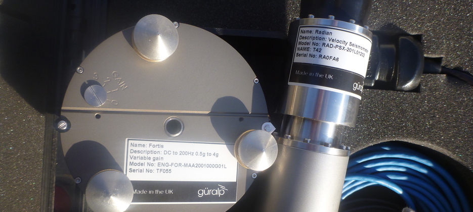
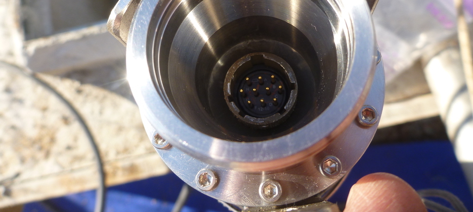
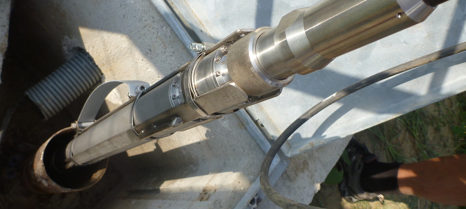
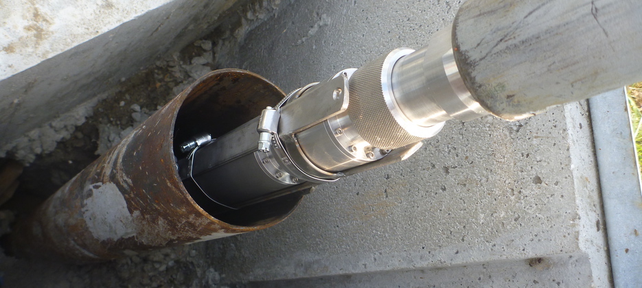
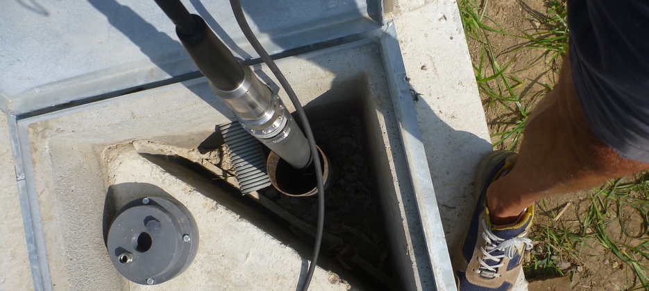
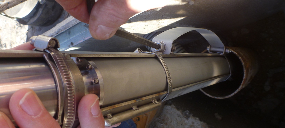
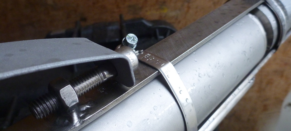
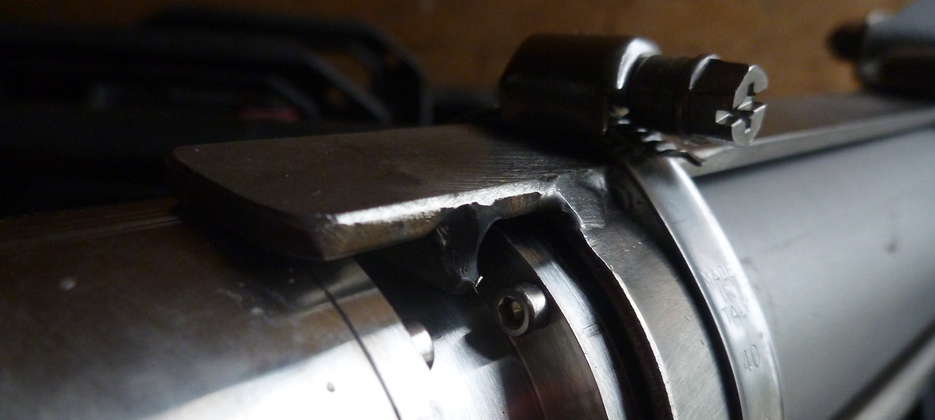
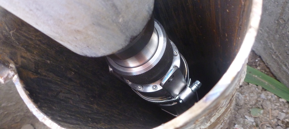
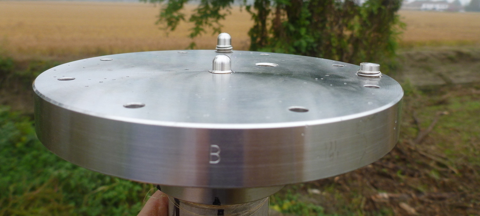
All stations of the RSCL are equipped with a seismometer placed in a well to improve the quality of the detected signal and an accelerometer placed on the surface. The figure shows a map of the RSCL with highlighted domains of detection adopted by the monitoring system, according to the definitions in the MiSE Guidelines.

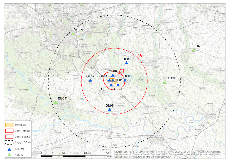
Map of the RSCL. The blue and green triangles indicate the stations of the RSCL and the Centralized National Seismic Network, respectively, used to integrate the surveys. The yellow area in the centre indicates the surface projection of the reservoir. The red lines indicate the perimeters of the Internal Domain (DI, thick line) and the Extended Domain (DE, thin line) of detection. The dotted line indicates the External Area, corresponding to a distance of 30 km from the storage site.

The RSCL records ground vibrations caused by the passage of seismic waves. Since the instruments are very sensitive, all ground vibrations are detected, both those caused by earthquakes and those generated by other sources such as the transit of vehicles (trains, trucks, etc.), the activity of industrial machinery, weather events (wind, thunder, etc.) or explosions of quarry or war ordnance. A proper analysis of the signal generally allows discrimination among the different types of events.

The RSCL is able to detect seismic events of interest to the community (therefore perceivable with different intensities by the population) as well as events that are not perceived by local residents, whether these events are strong and distant earthquakes (for example, those that occur in Japan and Chile) or very weak tremors that occur near the network.

The monitoring system continuously acquires signals from the stations of the network and automatically analyses them to recognize any anomalies; if these variations are found simultaneously at multiple stations, the system locates the origin and quantifies the extent. If certain conditions are met, the phenomenon is declared a “seismic event”. All these steps occur within seconds of the signal being recorded.

The automatic system is calibrated mainly to recognize earthquakes, but it may happen that different phenomena or false events due to the random simultaneity of signal variations are also identified as seismic events. Since the main purpose of the RSCL is to record microseisms that are not identified by regional or national networks, the system has been calibrated to very high sensitivity thresholds, which means many false events may be detected. For this reason, all automatic determinations are reviewed by an expert seismologist who analyses the automatically identified events, confirming whether they actually correspond to local natural earthquakes or events potentially related to the activity of the storage facility.

The ground vibrations recorded by the instruments are usually represented with graphs, called seismograms, which describe the movement of the ground (in displacement, velocity or acceleration) as time passes. From the seismograms, it is possible to evaluate where the seismic event occurred, how strong it was and some of its other characteristics.

In the past, seismograms were plotted on paper and visually analysed. Today, digitized data are stored on electronic media and analysed through special programs to be interpreted or represented on video or printed on paper.

By way of illustration, some seismograms are represented below, as they appear in real time in the Seismograms in near real time section of this website or after they are processed by the staff in charge of their interpretation.

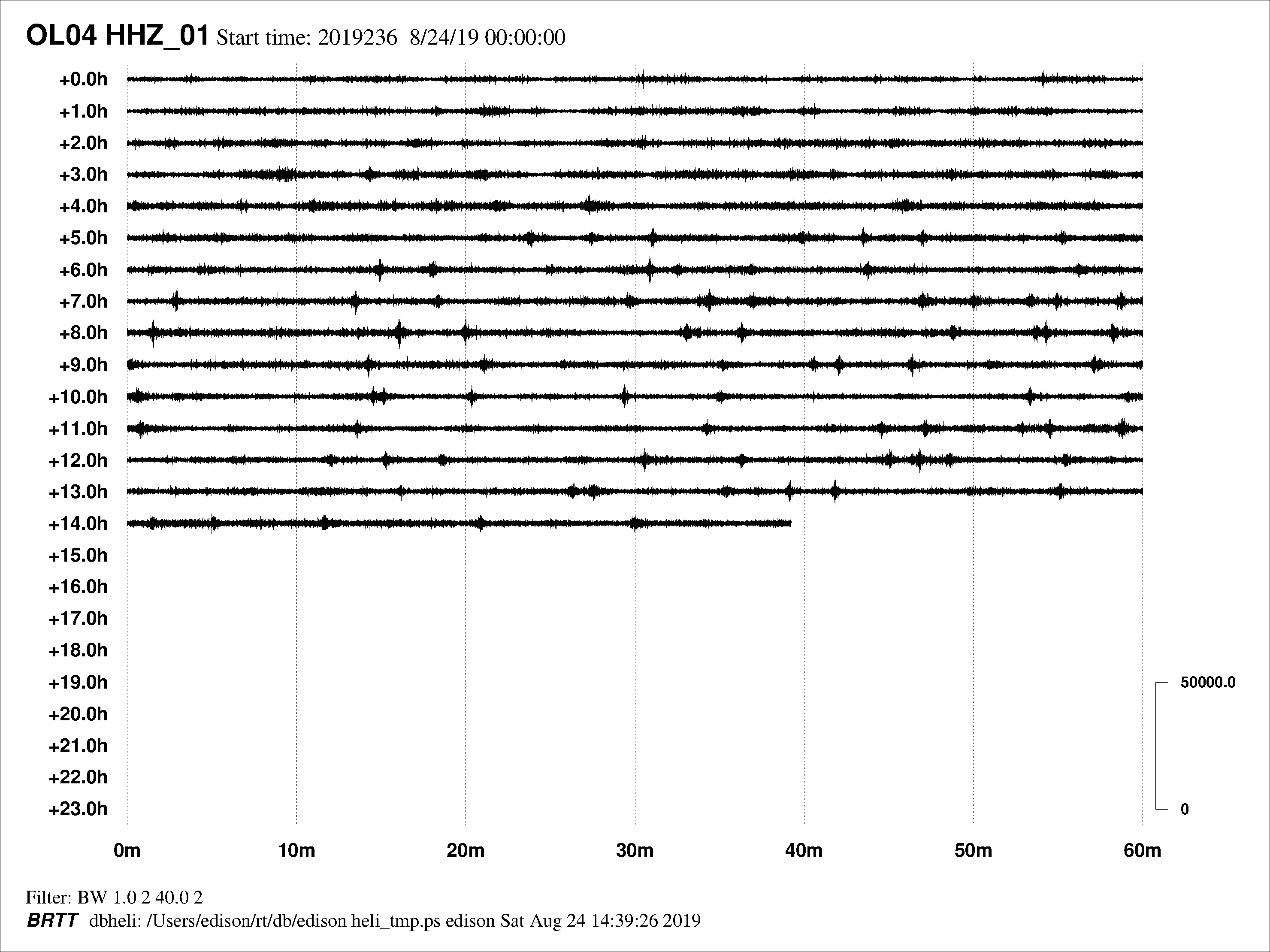
Daily recording from a station: Each line of the seismogram corresponds to one hour of recording. These representations are called "drumplots" or "helicorders" because they simulate what was formerly recorded by means of a trace imprinted on a rotating paper drum. The figure shows the recording of a single component of the ground motion (the position of a point in space is expressed by a Cartesian coordinate system) for an instrument that is acquiring data in "real time"; the trace then stops with the last data acquired by the instrument at the moment when the figure was produced (approximately 14:40). This type of visualization is also used to verify the correct functioning of the station.

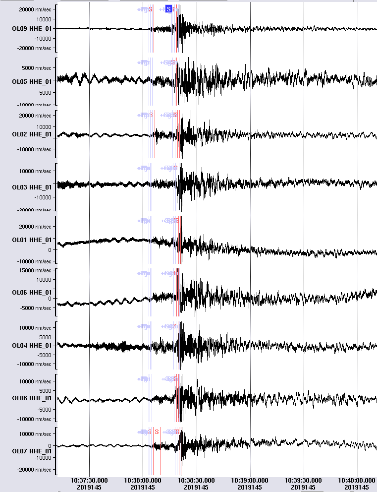
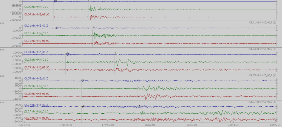
Recording of the same event by several stations: Seismograms indicate an interval of time limited to a few minutes. Each station can be represented by several tracks representing the three recorded spatial components: two horizontal and one vertical. Signal processing involves the use of filters (this is the case represented here) to remove or emphasize some frequency components. This representation is used to control and manually review the signal of an automatically identified event.

Below are some examples of signals recorded by RSCL related to different types of events. In order, these are as follows:
- seismograms related to a strong event that occurred in central Italy;
- seismograms from a strong distant event ("teleseism") that occurred in the Pacific Ocean;
- signals due to trains in transit;
- recordings of two local microearthquakes.

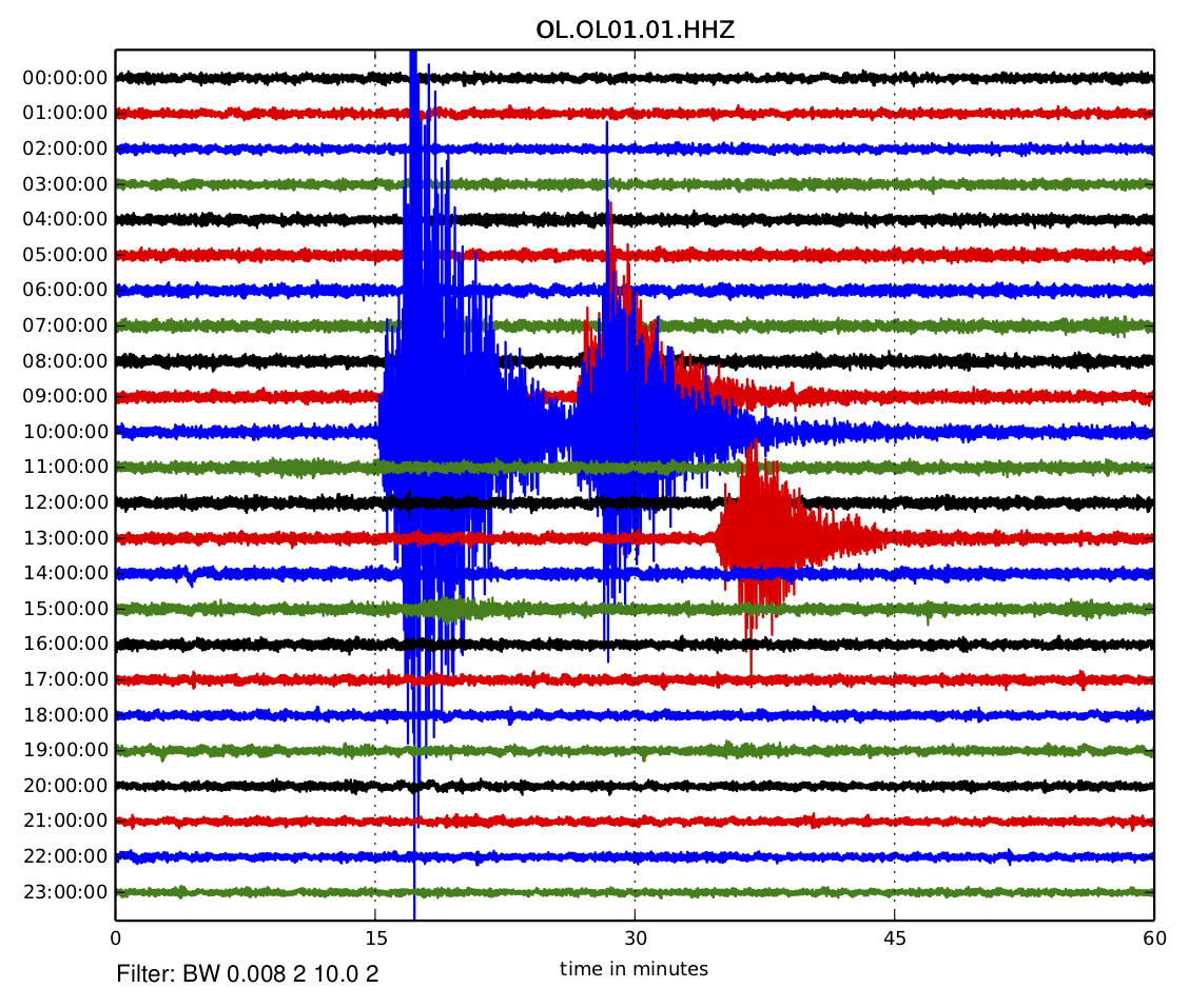
Registration at the OL01 station of the earthquakes with magnitude M>5 that occurred in central Italy on 18/1/2017. The different coloured tracks allow recognition of the overlapping signals; these events in central Italy tend not to be perceived by the population in the Lodi area. Note that by convention, the time of an earthquake is given by the Universal Co-ordinated Time (UTC), that is, the Greenwich meridian time (GMT). To correspond with Italian local time, it is necessary to add 1 hour (if solar time is in place) or 2 hours (if daylight saving time is in place) to the indicated value.

Registration at the OL04 station of a Mw 7.9 teleseism that occurred in the Pacific Ocean at 04:302:23.8 UTC on 22/1/2017 (source EMSC). These teleseisms are not perceived by the population.

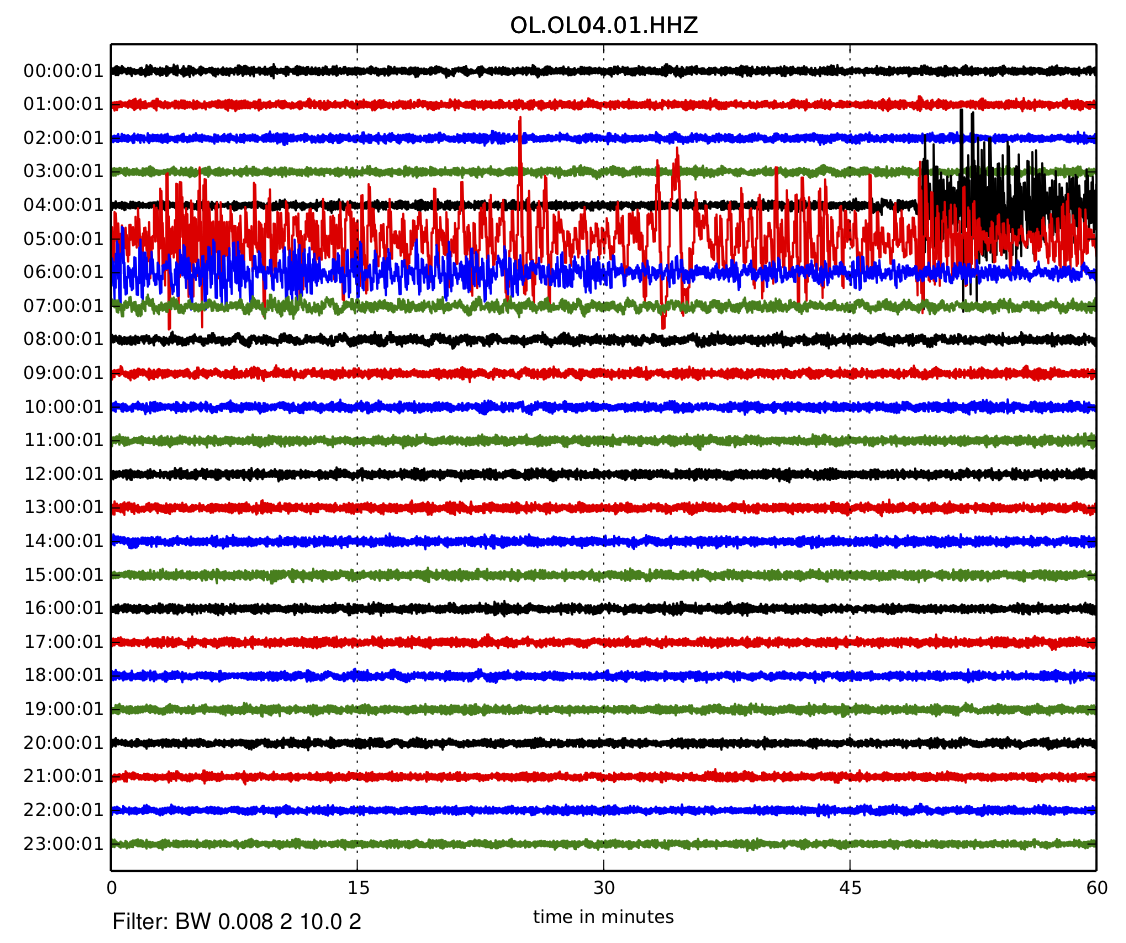
Recurring signals due to the passage of trains at the OL04 station on 30/1/2017. The OL04 station is located in Lodivecchio (Loc. Comasina) a few hundred metres from a high-speed train line. Despite the installation of the sensors at a depth of 75 metres, the seismic waves are identifiable. The vibrations of the ground from passing trains are sometimes perceivable by the population in the immediate vicinity of the railway line.

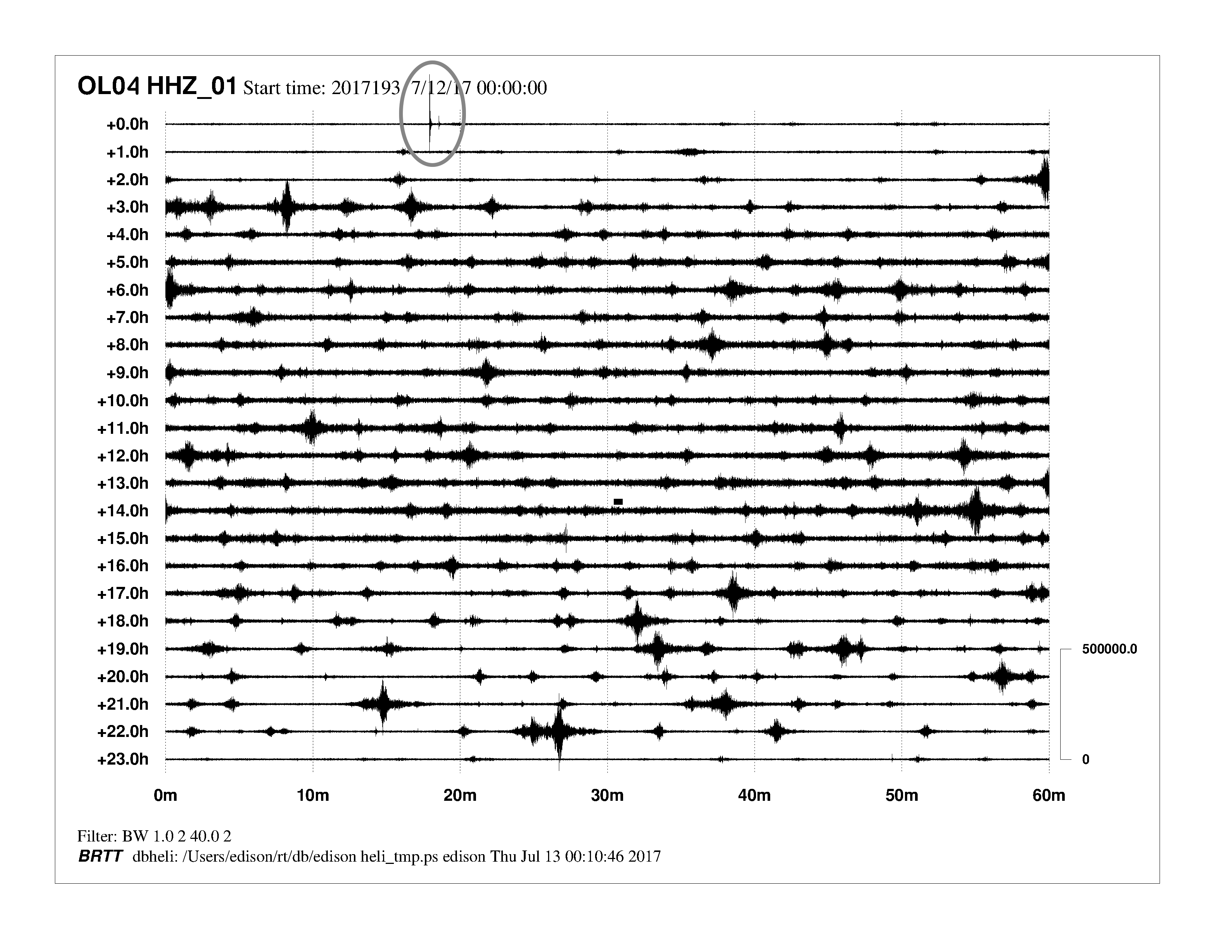
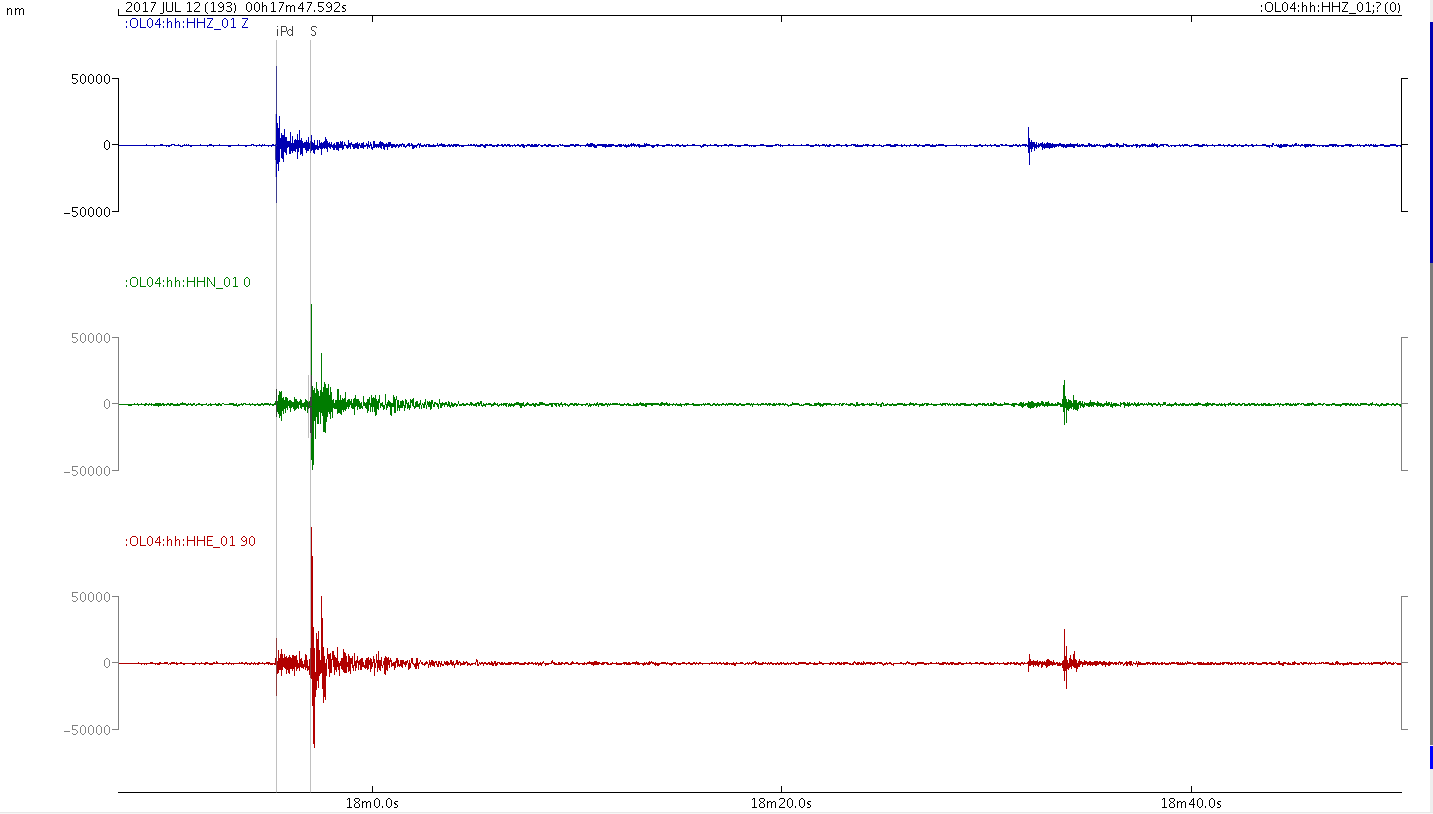
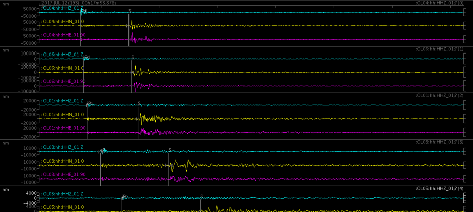
Registration at the OL04 station of two local microquakes with magnitude M≤1.0 that occurred on 12/7/2017 at 00:17:53 and 00:18:30. Top: daily helicorder-type recording of the vertical component at the same station (each line is one hour of recording); the signals of the two microquakes are enclosed within the grey ellipse. Bottom: one minute of recording (three-component seismograms) of the two microquakes. These events were not perceived by the population.

Seismic monitoring is used to identify and measure seismic events in the vicinity of or potentially of interest for the Cornegliano Laudense gas storage facility called "Cornegliano Stoccaggio".

If the vibration of the ground automatically identified within a few seconds by the system as a 'seismic event' corresponds to a local earthquake and has certain characteristics, the seismologist on call at OGS is alerted; within a few hours, the intervention and manual analysis of the data confirm or eliminate the event. The location and magnitude of the event is finally published on the page of the integrated monitoring system containing the "Recent Events". In the case of "attention conditions", the operator of the storage facility is notified promptly.

“Attention conditions" are situations in which there is an abnormal increase in microseismicity (in terms of magnitude and/or number of events detected) compared to conditions considered "normal" within the detection domains (the so-called seismic background). In this case, the seismologist in charge of monitoring intensifies the controls and analysis to obtain an accurate and updated picture of the detected microseismicity and verifies with the storage manager the activity carried out to establish or exclude any correlation between the storage facility and the detected microseismicity.

The Cornegliano Stoccaggio monitoring website provides complete information on the stations of the seismic network, graphs, technical and scientific documents and reports on the activity carried out. Further details can be found in the section with frequently asked questions (FAQ).

The survey system for geodetic monitoring consists of two components: a satellite component and an in situ component.
The satellite component uses data acquired by radar systems mounted on satellites orbiting several hundred kilometres from Earth (Figure 1), capable of providing high-resolution microwave images. These systems are called "SAR", which stands for synthetic aperture radar. Due to their longer wavelength than those of visible and infrared radiation, microwaves have the important property of penetrating through clouds, fog and possible coverings of ash or dust (for example, in the case of a volcanic eruption or collapse of a building); they are also independent of lighting conditions (day or night), thus allowing monitoring under any weather and environmental conditions.

The analysis of surface deformations in the Cornegliano Laudense area has been carried out using both archived SAR data, which allow observing the "past" history of ground movements in the area of interest, and recently acquired data, which monitor the current evolution of surface deformations.

As far as archived data are concerned, SAR images collected by the ERS-1/2 and ENVISAT sensors of the European Space Agency (ESA) over an area of approximately 95 km x 60 km, including the Cornegliano Laudense site, during the period 1993-2010, were used together. In particular, the deformation analysis was conducted using 141 images acquired by satellites along descending orbits (the satellite moves from north to south) and 76 along ascending orbits (the satellite moves from south to north).

With respect to monitoring, the analysis of surface deformations is carried out using data collected from the Sentinel-1 (S-1) constellation of the Copernicus European Programme, which is composed of twin sensors called S-1A and S-1B, which allow SAR images to be acquired every 6 days in the area of interest (Figure 1). In particular, 191 S-1 SAR data acquired from descending orbits and 200 from ascending orbits have been used over an area of approximately 190 km x 70 km that includes the site of Cornegliano Laudense from March 2015 through the present.

The analyses carried out based on satellite data are integrated with those conducted through the network of GNSS stations to bind the satellite measurements to some points located on the ground, for which the positions are known with precision.

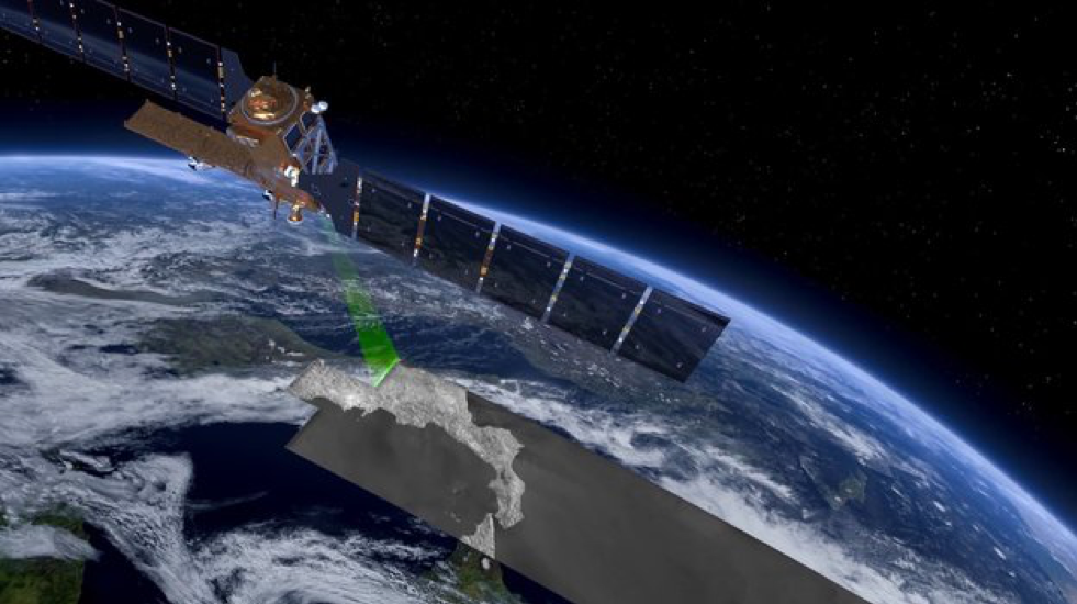
Figure 1 - Sentinel-1 sensors acquire microwave SAR images every 6 days over the area of interest, allowing continuous monitoring under all weather and environmental conditions.

The technique called “differential interferometry SAR” (DInSAR) allows the measurement of ground displacements (subsidence, slippage, etc.) with an accuracy on the order of centimetres and, in some cases, millimetres over very large areas (tens of thousands of square kilometres). The DInSAR methodologies basically "compare" pairs of SAR images acquired by one or more sensors from approximately the same position but at different times for a given area of the Earth's surface. If something has changed in the time interval between the two acquisitions, i.e., if ground deformation has occurred between the two sensor passes, this can be measured and displayed by means of a false colour map with a correspondence between colours and ground movement.

In addition, using advanced DInSAR techniques, by appropriately combining a sequence of SAR images acquired for the same area over time, the evolution of the surface deformation can be measured in the time interval considered. One of these techniques, called the small baseline subset (SBAS), allows the generation of ground deformation maps at medium and high spatial resolutions (tens of metres/metres) much denser spatially than traditional geodetic methods (geometric levelling campaigns or GPS measurements) and with increasing temporal frequencies.

It should be noted that the maps generated by DInSAR analysis measure the ground deformation projected along the sensor's line of sight (referred to in English as line of sight, LOS); in essence, these maps involve measuring how far a point on the ground moves away from or closer to the sensor along its LOS. However, taking advantage of acquisitions made from both descending and ascending orbits, the results of the respective analyses can be combined to generate both maps (Figure 1) and time series of deformation for the vertical and east-west components of the detected displacements.

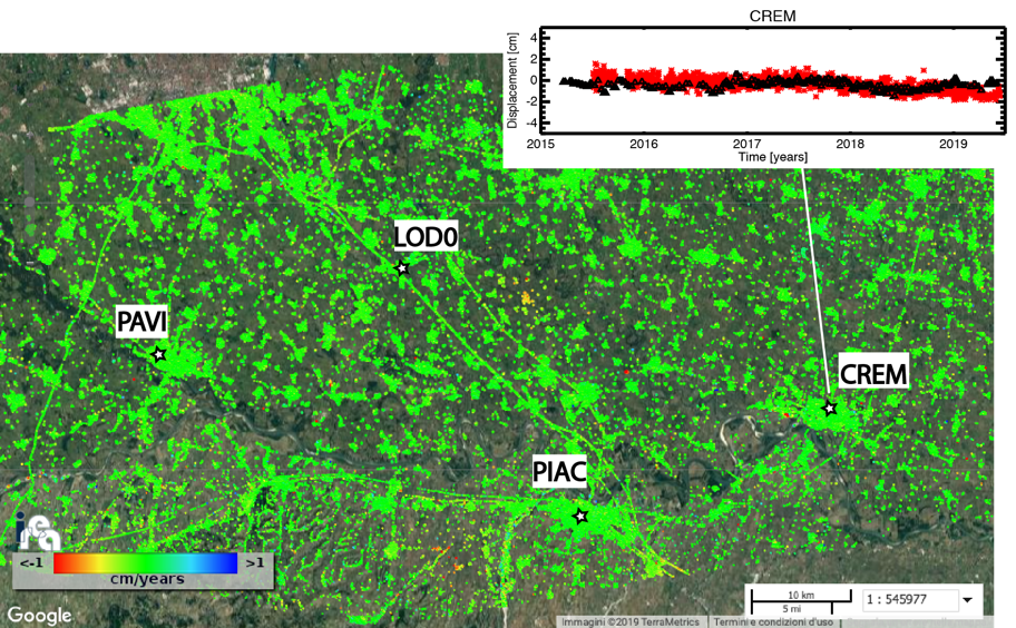
Figure 1 - Average LOS deformation velocity map of the terrain, expressed in cm/year, generated using SAR data acquired by the Sentinel-1 sensor, in the period 2015-2019, over an area of approximately 190 km x 70 km that includes the Cornegliano Laudense site, superimposed on the optical image of the area. The green colour represents undeformed areas, yellow and red areas have subsided, and blue and blue areas have been uplifted. In the box at the top right, for example, are represented the historical series of deformation at the GPS station in Cremona measured using DInSAR satellite data (black triangles) and GPS data (red asterisks), respectively. Note that the DInSAR time series are calculated for each coloured point on the map.

The main results of DInSAR analysis are the time series (also called historical series) of the ground deformation, typically measured in centimetres, and the related average deformation velocity maps calculated in cm/year, related to the time interval during which the data were acquired by the radar sensor and with a time frequency given by the time interval between two successive observations of the selected area on the ground.

The average ground deformation velocity maps are geocoded maps; therefore, they can be superimposed on existing maps of the area and are represented in false colours that correspond to the ground displacements. In these maps, only the points where the deformation measurement can be considered reliable are shown, and for each of these points, the historical deformation series is calculated.

The final spatial resolution of the ground deformation maps obtained by DInSAR analysis of Sentinel-1 data is approximately 30 m x 30 m, while their spatial extent is approximately 190 km x 70 km; the time sampling of the related historical deformation series is currently 6 days.

DInSAR measurements are differential measurements, i.e., relative measurements with respect to a point considered stable that is chosen as a reference. In our case, the reference point (also called the docking point) is a pixel located in the urban area of Pavia near a corresponding GPS station, which, as evidenced by the related GPS measurements, is not affected by deformation (see Figure 1).

The DInSAR analysis natively generates the measurement of the ground deformation projected along the sensor's line of sight (LOS) (see Figure 2 and Figure 3); however, by combining the DInSAR results produced by analysis carried out with acquisitions along ascending and descending orbits, it is possible to obtain measurements of the vertical and east-west components of the ground displacements (see Figure 4 and Figure 5).

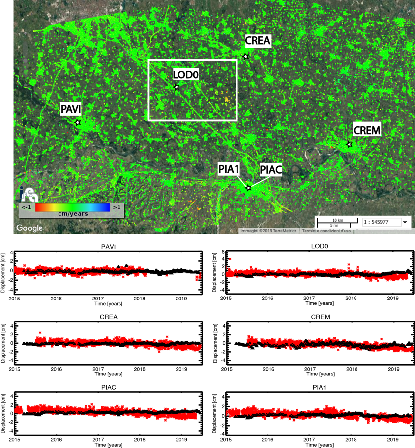
Figure 1 - LOS strain rate map, geocoded and expressed in cm/year, superimposed on an optical image of the area of interest. The image reflects the processing of S-1 data acquired from descending orbits in the period March 2015 - May 2019. The green colour represents undeformed areas, yellow and red areas have subsided, and blue and blue areas have been uplifted.
The graphs of the comparisons between the GPS deformation time series projected along the radar sensor's LOS (red asterisks) and those obtained through DInSAR data (black triangles) are also shown at the 6 GPS stations marked on the map by white stars. The white rectangle indicates the area analysed in detail in the figures below.

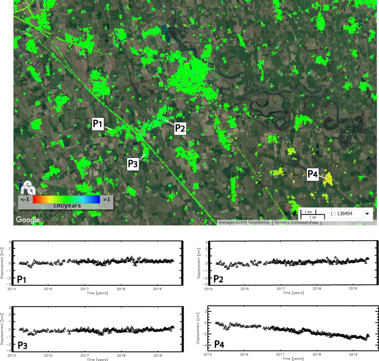
Figure 2 - Enlarged view of the Cornegliano Laudense area of the map of average surface deformation velocity along the LOS obtained by DInSAR analysis of S-1 data acquired from ascending orbits in the period March 2015 - May 2019, geocoded and expressed in cm/year, superimposed on an optical image of the area of interest.
The graphs show the temporal trend of the surface displacement along the LOS for three points located near Cornegliano Laudense (P1, P2 and P3) and one point located in the area of Turano Lodigiano (P4).

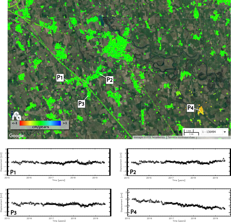
Figure 3 - Enlarged view of the Cornegliano Laudense area of the map of average surface deformation velocity along the LOS obtained through the DInSAR analysis of S-1 data acquired from descending orbits in the period March 2015 - May 2019, geocoded and expressed in cm/year, superimposed on an optical image of the area of interest.
The graphs show the temporal trend of the surface displacement along the LOS for three points located near Cornegliano Laudense (P1, P2 and P3) and one point located in the area of Turano Lodigiano (P4).

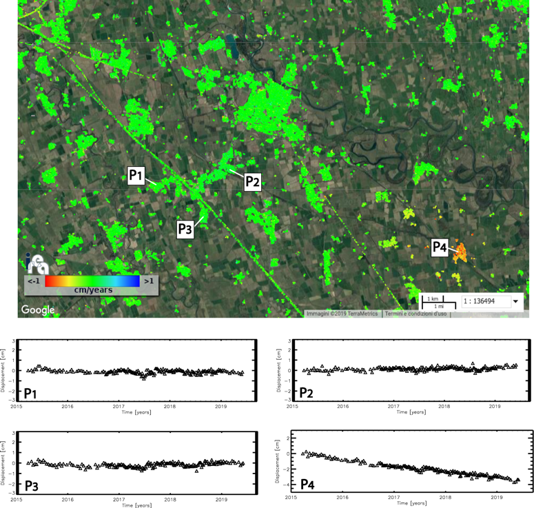
Figure 4 - Enlarged view of the Cornegliano Laudense area of the average rate map of the vertical component of the surface deformation obtained by appropriately combining the LOS DInSAR results related to data acquired from ascending and descending orbits shown in the previous figures, geocoded and expressed in cm/year, superimposed on an optical image of the area of interest. The graphs show the temporal trend of the vertical component of the ground displacement for three points located near Cornegliano Laudense (P1, P2 and P3) and one point located in the area of Turano Lodigiano (P4).

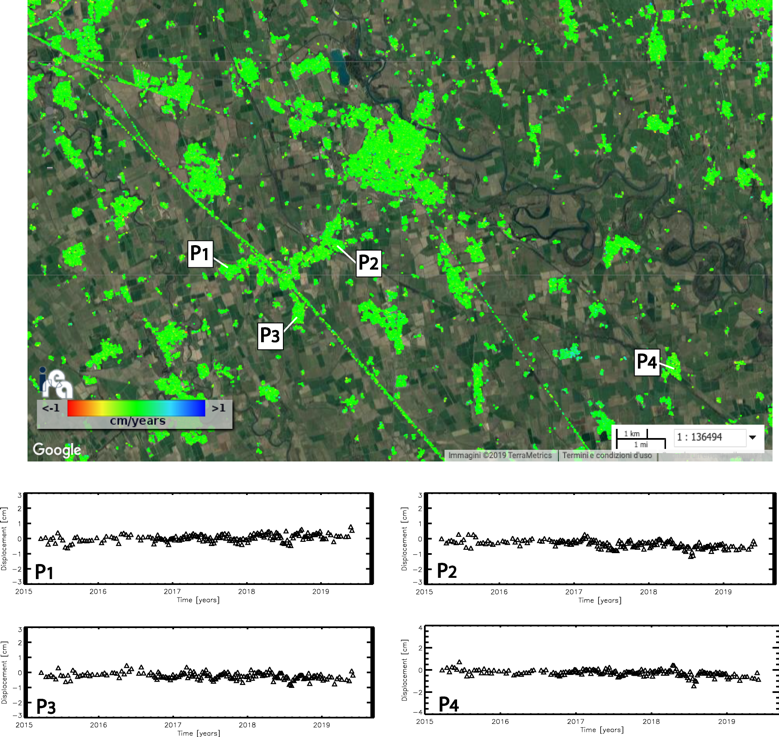
Figure 5 – Enlarged view of the Cornegliano Laudense area of the average rate map of the east-west component of the surface deformation obtained by suitably combining the LOS DInSAR results relative to the data acquired from ascending and descending orbits shown in the previous figures, geocoded and expressed in cm/year, superimposed on an optical image of the area of interest. The graphs show the temporal trend of the east-west component of the ground displacement for three points located near Cornegliano Laudense (P1, P2 and P3) and one point located in the area of Turano Lodigiano (P4).

The activities of extraction/storage of hydrocarbons and re-injection of fluids into the sub-soil can induce surface deformation phenomena. These deformation effects provide important information about the characteristics of the sub-surface phenomena from which they originated and their temporal evolution. Geodetic monitoring aims to provide information on both the temporal trend of ground deformation and its spatial distribution in the analysed area, highlighting any variations with respect to the background deformation scenario, i.e., prior to the underground exploitation activities.